An Introduction to ‘SSNbler’: Assembling Spatial
Stream Network (SSN) Objects in R
Erin E Peterson, Michael Dumelle, Alan R Pearse, Dan Teleki, and Jay M Ver Hoef
Source:vignettes/introduction.Rmd
introduction.RmdBackground
Data collected in streams frequently exhibit unique patterns of
spatial autocorrelation resulting from the branching network structure,
longitudinal (i.e., upstream/downstream) connectivity, directional water
flow, and differences in flow volume upstream of junctions (i.e.,
confluences) in the network (Peterson et al.,
2013). In addition, stream networks are embedded within
geographic (i.e., 2-D) space, with the terrestrial landscape often
having a strong influence on observations collected on the stream
network. Ver Hoef & Peterson (2010)
describe how to fit spatial statistical models on stream networks (i.e.,
spatial stream-network models) that capture the unique and complex
spatial dependencies inherent in streams. These stream network models
can be fit using the ‘SSN2’ R package (Dumelle, Peterson, Ver Hoef, Pearse, & Isaak,
2024). To use ‘SSN2’, however, users must provide the spatial,
topological, and attribute data in a specific format called an
SSN object. The ‘SSNbler’ R package, which
we introduce here, is an adaptation of the STARS ArcGIS toolset (Peterson & Ver Hoef, 2014) for the
R programming language. ‘SSNbler’ generates formats,
assembles, and validates SSN objects that can be used for
statistical modeling in ‘SSN2’.
In this vignette, we use ‘SSNbler’ to create the SSN
object MiddleFork04.ssn used by ‘SSN2’. First, we load
‘SSNbler’ into our current R session.
A few input datasets are included in the ‘SSNbler’ package:
-
MF_streams: Ansfobject withLINESTRINGgeometry representing a portion of the Middle Fork stream network in Idaho, USA. -
MF_obs: Ansfobject withPOINTgeometry containing observed summer mean stream temperature observations at 45 unique locations onMF_streams. -
MF_pred1km: Ansfobject withPOINTgeometry containing unsampled locations spaced at one-kilometer intervals throughoutMF_streams. This prediction dataset represents 175 locations where predictions of some response variable (i.e., temperature) may be desired. -
MF_CapeHorn: Ansfobject withPOINTgeometry containing 654 unsampled locations spaced at 10-meter intervals throughout Cape Horn Creek inMF_streams.
To provide context, the observed data in MF_obs will be
used to build statistical models and make predictions at the locations
in MF_pred1km and MF_CapeHorn using the
R package ‘SSN2’. Documentation for each dataset can be
found by running help(). For example, to learn more about
MF_streams, run
help("MF_streams", package = "SSNbler").
While these datasets come with ‘SSNbler’ and can be loaded via
data(), we focus here on a more realistic workflow for the
user. We start with a collection of spatial datasets installed alongside
‘SSNbler’ in the streamsdata folder that represent the
Middle Fork stream network. In streamsdata are GeoPackages
(more on this later) representing the stream network, observed data, and
prediction data (optional) required to create an SSN object. To prevent
‘SSNbler’ functions from reading and writing to this folder, we copy it
to R’s temporary directory and store the path to this folder:
copy_streams_to_temp()
path <- paste0(tempdir(), "/streamsdata")
Then we can read in the relevant data using st_read from
the ‘sf’ R package (Pebesma,
2018), which comes installed alongside ‘SSNbler’. Note that the
input data can be in any vector data format that can be imported into R
and stored as an sf object with LINESTRING or
POINT geometry (e.g., shapefile, GeoJSON, GeoPackage,
SpatiaLite, PostGIS).
library(sf)
MF_streams <- st_read(paste0(path, "/MF_streams.gpkg"))
MF_obs <- st_read(paste0(path, "/MF_obs.gpkg"))
MF_pred1km <- st_read(paste0(path, "/MF_pred1km.gpkg"))
MF_CapeHorn <- st_read(paste0(path, "/MF_CapeHorn.gpkg"))
Notice that the line (MF_Streams) and point features
(MF_obs, MF_pred1km, and
MF_CapeHorn) have LINESTRING and
POINT geometry types, which are required in ‘SSNbler’. If
these datasets had MULTILINESTRING or
MULTIPOINT geometry types, the ‘sf’ function
st_cast could be used to convert to the required geometry
types. All of the input data have an Albers Equal Area Conic projection
(EPSG 102003) and distances are measured in meters. It is important that
all input datasets have the same map projection, which must be a
projected coordinate system and not a geographic coordinate system
measured in Latitude and Longitude. The ‘sf’ function
st_transform can be used to reproject sf
objects in R.
We previously mentioned these data are stored in
streamsdata in a GeoPackage format. GeoPackages, like
shapefiles, are a way to store spatial data. We prefer GeoPackages over
shapefiles because they offer better support for high precision numeric
data compared to the traditional DBF (dBASE) format (used in
shapefiles), which limits the precision to 10 decimal places when
writing (not reading) to local files from R.
This is problematic because several important columns ‘SSNbler’ adds and
‘SSN2’ uses contain very small values ranging from zero to one. If these
columns are truncated it can lead to difficult-to-diagnose errors when
models are fit in ‘SSN2’. GeoPackages do not have this limitation. To
learn more about GeoPackages, visit here.
Before working with any of the input files, we visualize the stream network, observed sites, and prediction sites using the R package ‘ggplot2’ (Wickham, 2016).
library(ggplot2)
ggplot() +
  geom_sf(data = MF_streams) +
  geom_sf(data = MF_CapeHorn, color = "gold", size = 1.7) +
  geom_sf(data = MF_pred1km, colour = "purple", size = 1.7) +
  geom_sf(data = MF_obs, color = "blue", size = 2) +
  coord_sf(datum = st_crs(MF_streams))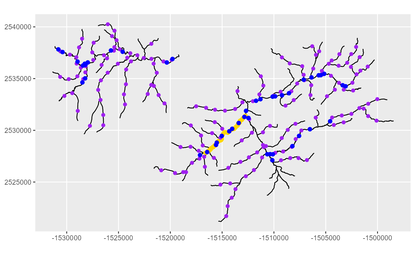
In the figure above, there are two subnetworks from
MF_Streams (black lines). Point features from
MF_obs (blue dots) and MF_pred1km (purple
dots) are found on both networks, while MF_CapeHorn point
features (yellow dots) are only found on one of the two networks.
The Landscape Network
‘SSNbler’ makes use of a data structure called a Landscape Network (LSN), which is a type of graph used to represent spatial context and relationships with additional geographic information (Theobald et al., 2006). In a LSN, streams are represented as a collection of directed edges, where the directionality is determined by the digitized direction of the line features. Nodes are located at the end points of edges (i.e., end nodes) and represent topologic breaks in the edges. For a more detailed description of the LSN, see Peterson & Ver Hoef (2014).
There are four topologically valid node categories in a LSN:
- Source: Water flow originates at these nodes and flows downstream. An edge that begins at a source node is called a headwater segment. Source nodes do not receive flow from any upstream edges.
- Outlet: Flow terminates at these nodes. This node is the most downstream point in an edge network. We refer to an edge that terminates at an outlet as an outlet segment. Note that a streams dataset may contain multiple subnetworks with associated outlets.
- Confluence: Multiple edges converge, or flow into, a single node.
- Pseudonode: One edge flows in and one edge flows out of a single node. While these nodes are not topologically problematic, an excessive number of pseudonodes can slow down geoprocessing operations for large datasets.
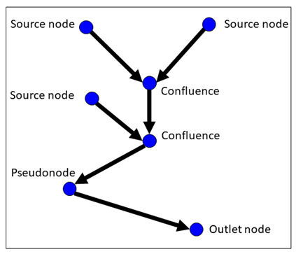
A landscape network (LSN). Nodes are denoted by blue circles, with the node category labelled. Edges are denoted by black arrows, with the arrow indicating flow direction (i.e., digitized direction).
Each edge is associated with two nodes, which correspond to the
upstream and downstream end nodes of the edge. When more than one edge
flows into or out of the node, they share a node. Thus, there
should always be a single node at the intersection of edges. If there is
more or less than one node at an intersection, it is a topological
error. If these errors are not corrected, the connectivity between line
features and the observed and prediction sites associated with them will
not be accurately represented in the SSN object or the
spatial statistical models subsequently fit to the data. In this
vignette, we assume that MF_streams has already been
checked and topologically corrected. Two tutorials have been created
with detailed instructions about identifying and correcting topological
errors in the LSN, as well as other topological restrictions that are
not permitted (please see ‘Correcting topological errors using SSNbler
and QGIS’ or ‘Correcting topological errors using SSNbler and ArcGIS
Pro’). These tutorials are available for download within the relevant
folders on GitHub at this
link.
Building the Landscape Network
The LSN is created using the lines_to_lsn() function,
which generally requires these arguments:
-
streams: Ansfobject withLINESTRINGgeometry that represents the stream network. -
lsn_path: A path to the directory in which the LSN output files will be stored. This directory will be created if it does not exist. -
check_topology: Logical indicating whether to check for topological errors instreams. -
snap_tolerance: Two nodes separated by a Euclidean distance \(\le\)snap_tolerancewill be assumed connected. Distance is measured in map units (i.e., projection units forstreams). -
topo_tolerance: Two nodes separated by a Euclidean distance \(\le\)topo_toleranceare flagged as potential topological errors in the network.
We create a LSN associated with MF_streams by
running
## Set path for new folder for lsn
lsn.path <- paste0(tempdir(), "/mf04")

edges <- lines_to_lsn(
  streams = MF_streams,
  lsn_path = lsn.path,
  check_topology = TRUE,
  snap_tolerance = 0.05,
  topo_tolerance = 20,
  overwrite = TRUE
)
The lines_to_lsn() function writes a minimum of five
files to lsn_path:
-
nodes.gpkg: A GeoPackage withPOINTgeometry features representing LSN nodes. It contains a unique node identifier column,pointid, and another column namednodecat, which contains the node type (pseudonode, confluence, source, outlet). -
edges.gpkg: A GeoPackage withLINESTRINGgeometry features representing LSN edges, which contains all of the columns instreamsand a unique edge (i.e., reach) identifier column namedrid. -
nodexy.csv: A comma-separated value (csv) file with thepointidand x and y coordinates for each node. -
noderelationships.csv: A csv file with three columns used to describe the directional relationship between nodes and edges. The columnridis the edge identifier, while thefromnodeandtonodecontain thepointidvalue for the upstream and downstream node, respectively. -
relationships.csv: A csv file that describes the directional relationship between edges using two columns namedfromedgeandtoedge, which contain the edgeridvalues.
Together these five files describe the geographic and topological relationships between edges in the network, while preserving flow direction.
When check_topology = TRUE, lines_to_lsn()
also checks the topology of the network. When potential topological
errors are identified, they are saved at the location specified by
lsn_path as a GeoPackage named
node_errors.gpkg with POINT geometry.
It is important to pay attention to the output messages from
lines_to_lsn() that are printed to the R
console. In this example, the message is
No obvious topological errors detected and node_errors.gpkg was NOT created.
This suggests that the LSN edges are error-free, but it is still a good
idea in practice to visually assess maps of the node
nodecat values to look for obvious errors, as described in
the topology editing tutorials mentioned previously. If
node_errors.gpkg was created, then potential topological
errors were identified, which must be checked and corrected before
moving on to the next spatial processing steps.
Incorporating Sites Into the Landscape Network
After creating the error-free LSN using lines_to_lsn(),
observed and prediction datasets are incorporated into the LSN using
sites_to_lsn(). The function snaps (i.e., moves) point
locations to the closest edge location and generates new information
describing the topological relationships between edges and sites in the
LSN. sites_to_lsn() generally requires these arguments:
-
sites: Ansfobject withPOINTgeometry that contains the observed or prediction locations. -
edges: Ansfobject containing the edges in the LSN generated usinglines_to_lsn(). -
snap_tolerance: A numeric distance in map units. If the distance to the nearest edge feature is less than or equal tosnap_tolerance, sites are snapped to the relevant edge. If the distance to the nearest edge feature is greater thansnap_tolerance, the point feature is not snapped to an edge or included in the output. -
save_local: IfTRUE(the default), the snapped sites are written tolsn_pathwith name specified byfile_name. -
lsn_path: A path to the directory where the LSN created vialines_to_lsn()is stored. -
file_name: Output file name for the snapped sites, which are saved inlsn_pathin GeoPackage format.
We run sites_to_lsn for the MF_obs
(observed) data:
obs <- sites_to_lsn(
  sites = MF_obs,
  edges = edges,
  lsn_path = lsn.path,
  file_name = "obs",
  snap_tolerance = 100,
  save_local = TRUE,
  overwrite = TRUE
)
In the code above, sites_to_lsn() writes a GeoPackage
named obs.gpkg to lsn_path and also returns
these snapped sites as an sf object named obs.
The new dataset contains the original columns in sites and
three new columns:
-
rid: The edgeridvalue where the snapped site resides. -
ratio: Describes the site location on the edge. It is calculated by dividing the length of the edge found between the downstream end node and the site location by the total edge length. -
snapdist: The Euclidean distance in map units the site was moved.
The rid value provides information about where a site is
in relation to all of the other edges and sites in an LSN, while the
ratio value can be used to identify where exactly
a site is on the edge. Note that the sites_to_lsn function
must be run for each dataset, even if the site locations already
intersect edge features.
It is important to pay attention to the message output in the
R console because it indicates how many of the sites
were successfully snapped to the LSN. In this case, the message says
Snapped 45 out of 45 sites to LSN. If some sites were not
snapped, the snap_tolerance value should be increased until
all sites are snapped. The snapdist column can then be used
to identify sites that were moved relatively large distances to ensure
they were snapped to the correct edge.
Prediction datasets (optional) represent spatial locations where
predictions from a spatial stream-network model may be desired. They are
optional, but must also be incorporated into the LSN using
sites_to_lsn() before predictions can be made using a
fitted model. We add the MF_pred1km and
MF_capehorn prediction datasets to the LSN by running
preds <- sites_to_lsn(
  sites = MF_pred1km,
  edges = edges,
  save_local = TRUE,
  lsn_path = lsn.path,
  file_name = "pred1km.gpkg",
  snap_tolerance = 100,
  overwrite = TRUE
)

capehorn <- sites_to_lsn(
  sites = MF_CapeHorn,
  edges = edges,
  save_local = TRUE,
  lsn_path = lsn.path,
  file_name = "CapeHorn.gpkg",
  snap_tolerance = 100,
  overwrite = TRUE
)
Note that a LSN can contain an unlimited number of prediction
datasets, but only one set of observations. The
sites_to_lsn function must be run separately for every
observed and prediction dataset. While this may at first seem tedious,
it provides the user the opportunity to examine each output dataset
individually, ensuring that all sites are snapped to the LSN and the
correct edge feature.
The lines_to_lsn and sites_to_lsn functions
are used to produce a topologically corrected LSN containing edges,
observed sites, and prediction sites (optional). This LSN provides the
foundation for all of the remaining spatial data processing steps and
the spatial statistical models. Creating the LSN is often the most
time-consuming step in the spatial statistical modeling workflow,
especially if the edges or sites contain a large number of features or
the stream network has many topological errors. However, it is critical
that the spatial and topological relationships are accurately
represented in the LSN and the subsequent spatial statistical
models.
The LSN created using lines_to_lsn() and
sites_to_lsn() is stored in memory and also in a local
folder defined using lsn_path. The LSN contains at least
six components. The edges, nodes, and observed sites contain the spatial
features and attribute data within each dataset, while the
three tables (nodexy, noderelationships, and relationships) describe the
relationships between edges and sites. These tables are not
stored in memory but are accessed by subsequent ‘SSNbler’ functions.
Prediction datasets may also be included in the LSN if desired. By
default, all ‘SSNbler’ functions will update the files stored locally in
lsn_path and return an updated sf
object. However, the save_local argument can be set to
FALSE in most functions if the user would prefer not to save results
locally.
| LSN Component | In Memory | Local LSN Directory |
|---|---|---|
| edges | sf object, LINESTRING geometry |
GeoPackage |
| observed sites | sf object, POINT geometry |
GeoPackage |
| prediction sites (optional) | sf object, POINT geometry |
GeoPackage |
| nodes | GeoPackage | |
| nodexy table | csv file | |
| noderelationships table | csv file | |
| relationships table | csv file |
Once the LSN has been created, the next steps are to calculate the information needed to fit spatial stream-network models.
Calculating Upstream Distance
The “upstream distance” represents the hydrologic distance (i.e., distance between locations when movement is restricted to the stream network) between the network outlet and each feature. For an edge, the distance is measured to the upstream end node of the line feature. The upstream distance for the \(j\)th edge, \(upDist_j\), is:
\[ upDist_j = \sum_{k \in D_j}{L_k}, \]
where \(L_j\) is the length of each edge and \(D_j\) is the set of edges found in the path between the network outlet and the \(j\)th edge, including the \(j\)th edge.
The upstream distance for each edge is calculated using the
updist_edges() function, which generally requires these
arguments:
-
edges: Ansfobject containing the edges in the LSN generated usinglines_to_lsn(). -
save_local: A logical indicating whether the updated edges should be saved tolsn_pathin GeoPackage format. Default is TRUE. -
lsn_path:LSNpathname whereedgesandrelationships.csvare stored locally. -
calc_length: A logical indicating whether a column representing line length should be calculated and added toedges. It is important to setcalc_length = TRUEif the edge features have been edited.
edges <- updist_edges(
  edges = edges,
  save_local = TRUE,
  lsn_path = lsn.path,
  calc_length = TRUE
)

names(edges) ## View edges column names
#> [1] "rid" "COMID" "GNIS_NAME" "REACHCODE" "FTYPE"
#> [6] "FCODE" "AREAWTMAP" "SLOPE" "rcaAreaKm2" "h2oAreaKm2"
#> [11] "Length" "upDist" "geom"Two columns are added to edges and saved in edges.gpkg.
Length represents the length of each edge in map units and
upDist is the upstream distance for each edge.
For sites, the upstream distance is calculated a little differently because it is the hydrologic distance between the network outlet and each site. The upstream distance for site \(i\), \(upDist_i\), is calculated as: \[ upDist_i = r_i L_i + \sum_{k \in D^*_j}{L_k}, \]
where \(r_i\) is the
ratio value for \(site_i\), \(L_i\) is the length of the edge \(site_i\) resides on, and \(D^*_j\) is the set of edges found in the
path between the network outlet and \(site_i\), excluding the edge \(site_i\) resides on.
Upstream distance is calculated for each site using the
updist_sites() function, which generally requires a few
arguments:
-
sites: A named list of one or moresfobjects withPOINTgeometry, which have been incorporated into the LSN usingsites_to_lsn(). -
edges:Ansfobject representing edges that have been processed usinglines_to_ssn()andupdist_edges(). -
length_col: The name of the column inedgesthat represents edge length. -
save_local: A logical indicating whether the updated sites should be saved tolsn_pathin GeoPackage format. Default is TRUE. -
lsn_path: The LSN pathname where thesitesandedgesGeoPackages reside. Must be specified ifsave_localis TRUE.
site.list <- updist_sites(
  sites = list(
    obs = obs,
    pred1km = preds,
    CapeHorn = capehorn
  ),
  edges = edges,
  length_col = "Length",
  save_local = TRUE,
  lsn_path = lsn.path
)

names(site.list) ## View output site.list names
#> [1] "obs" "pred1km" "CapeHorn"
names(site.list$obs) ## View column names in obs#> [1] "rid" "STREAMNAME" "COMID" "AREAWTMAP" "SLOPE"
#> [6] "ELEV_DEM" "Source" "Summer_mn" "MaxOver20" "C16"
#> [11] "C20" "C24" "FlowCMS" "AirMEANc" "AirMWMTc"
#> [16] "rcaAreaKm2" "h2oAreaKm2" "ratio" "snapdist" "geom"
#> [21] "upDist"The data stored in upDist are later used to calculate
the directional hydrologic distances between observed and prediction
locations in the ‘SSN2’ package. If we plot the edges and observations,
assigning color based on the upDist column, it is apparent
that the upstream distance increases from the outlet to headwater
streams, as expected.
ggplot() +
  geom_sf(data = edges, aes(color = upDist)) +
  geom_sf(data = site.list$obs, aes(color = upDist)) +
  coord_sf(datum = st_crs(MF_streams)) +
  scale_color_viridis_c()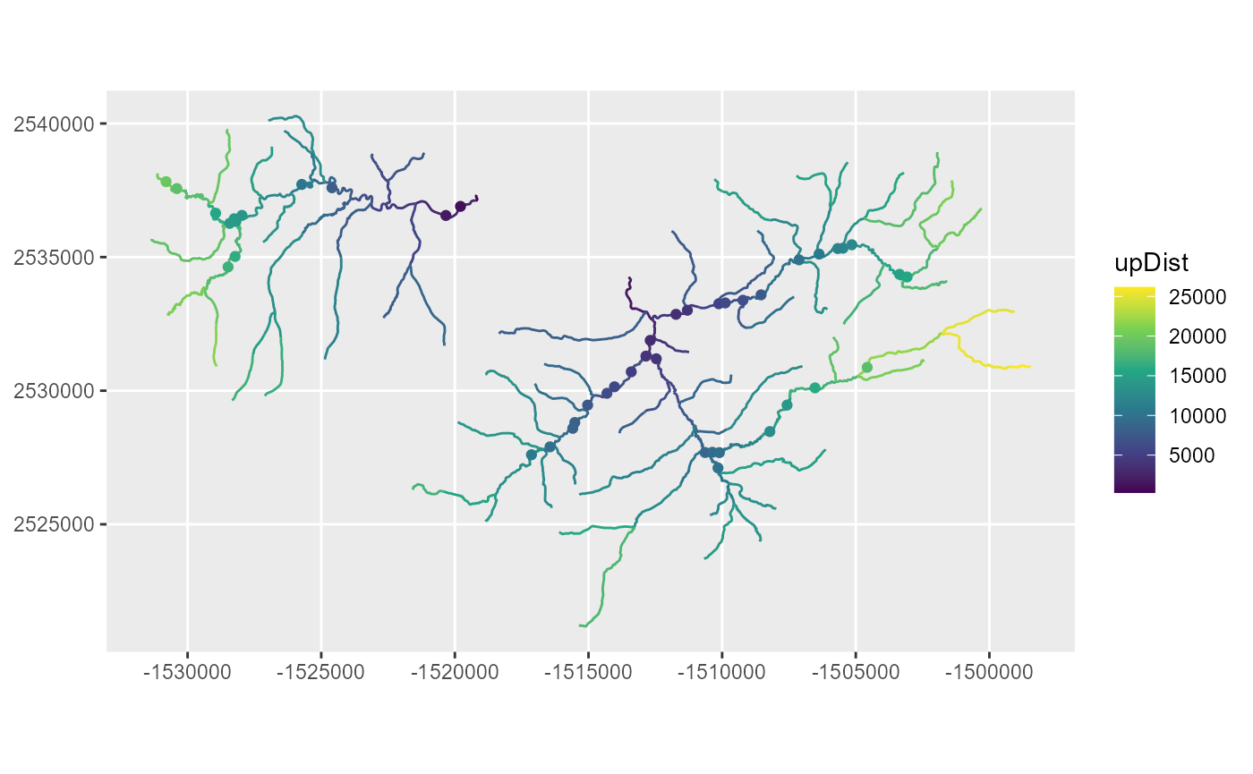
Calculating Additive Function Values (AFVs)
Spatial weights are used to split the tail-up covariance function upstream of network confluences, which allows for the disproportionate influence of one upstream edge over another (e.g., a large stream channel converges with a smaller one) on downstream values. Calculating the spatial weights is a three-step process: 1) calculating the segment proportional influence (PI), 2) calculating the additive function values (AFVs), and 3) calculating the spatial weights. Steps 1) and 2) are undertaken in ‘SSNbler’, while Step 3) is calculated in the package ‘SSN2’ when spatial stream-network models are fit.
The segment PI for each edge, \(\omega_j\), is defined as the relative influence of the \(j\)th edge feature on the edge directly downstream. In the following example, \(\omega_j\) is based on cumulative watershed area for the downstream node of each edge, \(A_j\), which is used as a surrogate for flow volume. However, simpler measures could be used, such as Shreve’s stream order (Shreve 1966) or equal weighting, as long as a value exists for every line feature in edges (i.e., missing data are not allowed). It is also preferable to use a column that does not contain values equal to zero, which we explain in more detail below.
When two edges, denoted \(j\) and \(k\), converge at a node, the segment PI for the \(j\)th edge is:
\[ \omega_j=\frac{A_j}{A_j + A_k}. \]
Notice that the segment PI values are ratios. Therefore, the sum of the PI values for edges directly upstream of a single node always sum to one. Also note that \(\omega_j=0\) when \(A_j=0\).
The AFVs for the \(j\)th edge, \(AFV_j\), is equal to the product of the segment PIs found in the path between the edge and the network outlet, including edge \(j\) itself.
\[ AFV_j = \prod_{k \in D_j}{\omega_k}. \]
If \(\omega_j=0\), the AFV values for edges upstream of the \(j\)th edge will also be equal to zero. This may not be problematic if the \(j\)th edge is a headwater segment without an observed site. However, it can have a significant impact on the covariance structure of the tail-up model when the \(j\)th edge is found lower in the stream network.
AFVs are calculated for every edge in the network using
afv_edges(), which generally requires these arguments:
-
edges: Ansfobject representing edges that has been processed usinglines_to_lsn(). -
lsn_path: The LSN pathname where theedgesreside. -
infl_col: The name of the numeric column in edges used to calculate the segment PI for each edge feature. Missing values are not allowed. -
segpi_col: The name of the new column in edges where segment PI values are stored. -
afv_col: The name of the new column in edges where AFVs are stored. -
save_local: A logical indicating whether the updated edges should be saved tolsn_pathin GeoPackage format. Default is TRUE.
Note that we use a variable representing cumulative watershed area
that is already present in edges (h2oAreaKm2)
to create the segment PI values:
summary(edges$h2oAreaKm2) ## Summarize and check for zeros#> Min. 1st Qu. Median Mean 3rd Qu. Max.
#> 0.0036 2.4534 5.9877 22.6237 28.2600 209.8989
edges <- afv_edges(
  edges = edges,
  infl_col = "h2oAreaKm2",
  segpi_col = "areaPI",
  afv_col = "afvArea",
  lsn_path = lsn.path
)

names(edges) ## Look at edges column names
#> [1] "rid" "COMID" "GNIS_NAME" "REACHCODE" "FTYPE"
#> [6] "FCODE" "AREAWTMAP" "SLOPE" "rcaAreaKm2" "h2oAreaKm2"
#> [11] "Length" "upDist" "areaPI" "afvArea" "geom"
summary(edges$afvArea) ## Summarize the AFV column#> Min. 1st Qu. Median Mean 3rd Qu. Max.
#> 0.004709 0.026168 0.066095 0.160335 0.169575 1.000000The AFVs are a product of ratios, which means that the AFVs are always between zero and one (\(0 \le AFV \le 1\)). The AFV for the most downstream edge in a network will always be one. If AFVs do not meet this requirement, then an error has occurred.
Once the AFVs have been added to edges, they can be calculated for the observations and (if relevant) prediction sites. The AFV for any site is equivalent to the AFV of the edge it resides on. If there are multiple sites on a single edge feature, their AFVs will be equal. Also note that when the AFV for the \(i\)th site is zero, the covariance between data collected at the \(i\)th site and every other site will also be zero. For more on additive function values, see Ver Hoef & Peterson (2010) and Peterson & Ver Hoef (2010).
The afv_sites function is used to create an AFV column
in a list of observed and prediction sites. The inputs include:
-
sites: A named list of one or moresfobjects withPOINTgeometry, which have been incorporated into the LSN usingsites_to_lsn(). -
edges: Ansfobject representing edges, which containsafv_colcreated usingedges_afv(). -
afv_col: The name of the column containing the AFVs inedges. A new column with this name will be added tosites. -
save_local: IfTRUE(the default), the updated sites are written tolsn_path. -
lsn_path: A path to the directory where the LSN created vialines_to_lsn()is stored. Required whensave_local = TRUE.
site.list <- afv_sites(
  sites = site.list,
  edges = edges,
  afv_col = "afvArea",
  save_local = TRUE,
  lsn_path = lsn.path
)

names(site.list$pred1km) ## View column names in pred1km
#> [1] "rid" "COMID" "AREAWTMAP" "SLOPE" "ELEV_DEM"
#> [6] "FlowCMS" "AirMEANc" "AirMWMTc" "rcaAreaKm2" "h2oAreaKm2"
#> [11] "ratio" "snapdist" "upDist" "afvArea" "geom"
summary(site.list$pred1km$afvArea) ## Summarize AFVs in pred1km and look for zeros#> Min. 1st Qu. Median Mean 3rd Qu. Max.
#> 0.009894 0.031219 0.047469 0.104969 0.112882 1.000000Each sf dataset in sites.list now has an
AFV column, afvArea, which was generated based on
cumulative watershed area. All AFVs should meet the requirement that
they are between zero and one.
Assembling the SSN Object
The last data processing step is to assemble the SSN
object using the ssn_assemble function.
The key arguments in ssn_assemble() include:
-
edges: Ansfobject representing edges that has been processed usinglines_to_lsn(),updist_edges(), andafv_edges(). -
lsn_path: The LSN pathname where theedgesand all observation and prediction site datasets reside. -
obs_sites:Optional. A singlesfobject representing observed sites, which has been processed usingsites_to_lsn(),updist_sites(), andafv_sites(). Default is is NULL. -
preds_list: Optional. A named list of one or moresfobjects representing prediction site datasets that have been processed usingsites_to_lsn(),updist_sites(), andafv_sites(). Default is NULL. -
ssn_path: The path to a local directory where the output files will be saved. A.ssnextension will be added if it is not included. -
import: Logical indicating whether the output files should be imported and returned as anSSNobject. -
check: Logical indicating whether the validity of theSSNobject should be checked usingssn_check(). Default is TRUE. -
afv_col: Character vector containing the names of the AFV columns that will be checked whencheck = TRUE. Columns must be present inedges,obs_sites, andpreds_list, if they are included.
mf04_ssn <- ssn_assemble(
  edges = edges,
  lsn_path = lsn.path,
  obs_sites = site.list$obs,
  preds_list = site.list[c("pred1km", "CapeHorn")],
  ssn_path = paste0(path, "/MiddleFork04.ssn"),
  import = TRUE,
  check = TRUE,
  afv_col = "afvArea",
  overwrite = TRUE
)
#>
#>
#> SSN object is valid: TRUE
class(mf04_ssn) ## Get class#> [1] "SSN"
names(mf04_ssn) ## print names of SSN object#> [1] "edges" "obs" "preds" "path"
names(mf04_ssn$preds) ## print names of prediction datasets#> [1] "pred1km" "CapeHorn"The outputs of ssn_assemble() are stored locally in a
directory with a .ssn extension and in memory as an object
of class SSN when import = TRUE. At a minimum,
the new .ssn directory will contain:
-
edges.gpkg: edges in GeoPackage format -
sites.gpkg: observed sites in GeoPackage format (if included) -
Prediction datasets: (e.g.,CapeHorn.gpkgandpred1km.gpkg) in GeoPackage format (if included) -
netIDx.dat files: one text file for each unique subnetwork in edges containing information describing the topological relationships between edges.
When import = TRUE, the spatial data stored in the
.ssn directory are imported into R and
stored in memory as an SSN object. The
netIDx.dat files are combined behind the scenes into an
SQLite database named binaryID.db, which is saved in the
.ssn directory. Most users will not need to access the
binaryID.db or the netIDx.dat files, but a
more detailed description about how the topological relationships are
stored can be found in Peterson & Ver Hoef
(2014).
The SSN object itself is a list containing four
elements:
-
edges: Ansfobject representing edges. -
obs: Ansfobject of observed sites. -
preds: Named list ofsfobjects representing prediction site datasets. -
path: Character string describing the path to the.ssnwhere theSSNcomponents are stored locally.
Including observed sites is optional in ssn_assemble and
when they are missing obs will contain NA
rather than an sf object. Most users will likely include
observations because they are needed to fit spatial statistical
stream-network models. Nevertheless, this option provides the
flexibility to include additional functionality in future ‘SSNbler’
versions. More specifically to create an SSN object based
on existing stream network data, generate artificial observed locations
at various locations throughout the network, and simulate data at those
locations using the ‘SSN2’ function ssn_simulate.
The path element provides a critical link between the
.ssn directory and the SSN object stored in R.
This is important because the ‘SSN2’ package reads and writes data to
this directory during the spatial stream-network modeling workflow.
The ssn_assemble function also adds several important
columns to the edges, obs, and prediction datasets.
-
edges:-
netID: A unique network identifier
-
-
obsandpreds:-
netIDThe network identifier value for the edge the site resides on -
pid: A unique identifier for each measurement (i.e., point feature). -
locID: A unique identifier for each location. Note that repeated measurements at a site will have the samelocIDvalue, but differentpidvalues.
-
A netgeom (short for network geometry) column is also
added to each of the sf objects stored within an SSN
object. The netgeom column contains a character string
describing the position of each line (edges) and point
(obs and preds) feature in relation to one
another. The format of the netgeom column differs depending
on whether it is describing a feature with LINESTRING or
POINT geometry. For edges, the format of
netgeom is
\[ \texttt{ENETWORK (netID rid upDist)}, \] and for sites \[ \texttt{SNETWORK (netID rid upDist ratio pid locID)}. \]
The information stored in these columns is used to keep track of the
spatial and topological relationships in the network. The data used to
define netgeom is stored in the edges, observed sites, and
prediction sites datasets. We store an additional copy of this critical
information as text in the netgeom column because it
reduces the chances that users will unknowingly make changes to these
data, which in turn could change how relationships are represented in
spatial stream-network models.
Plotting an SSN Object
The ‘SSNbler’ and ‘SSN2’ packages do not include generic plotting
functions for SSN objects because the functionality is
already available in the package ‘ggplot2’. As an example, we create a
plot of the SSN object. The edges are displayed in blue,
with the linewidth proportional to cumulative watershed area column,
h2oAreaKm2. The summer stream temperature observations
(Summer_mn) are shown using the viridis color palette, with
pred1km locations shown as smaller white dots:
ggplot() +
  geom_sf(
    data = mf04_ssn$edges,
    color = "medium blue",
    aes(linewidth = h2oAreaKm2)
  ) +
  scale_linewidth(range = c(0.1, 2.5)) +
  geom_sf(
    data = mf04_ssn$preds$pred1km,
    size = 1.5,
    shape = 21,
    fill = "white",
    color = "dark grey"
  ) +
  geom_sf(
    data = mf04_ssn$obs,
    size = 1.7,
    aes(color = Summer_mn)
  ) +
  coord_sf(datum = st_crs(MF_streams)) +
  scale_color_viridis_c() +
  labs(color = "Temperature", linewidth = "WS Area") +
  theme(
    legend.text = element_text(size = 8),
    legend.title = element_text(size = 10)
  )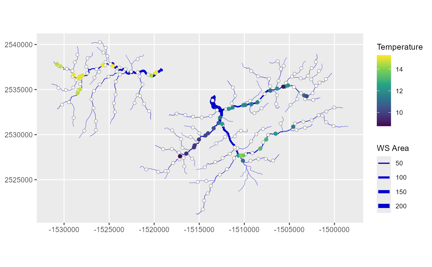
Mean summer stream temperature (Temperature) and cumulative watershed area (WS AREA) for the Middle Fork stream network. Prediction locations are white circles.
Notice the different ways the sf objects for the edges, obs, and
pred1km datasets are accessed in the SSN object and used
for plotting in the calls to geom_sf. Any valid plotting
function for sf objects and ggplot in general can be used to create
attractive plots of SSN object components.
Incorporating Data Into an sf or SSN Object
The edges, observations, and prediction locations are stored as
sf objects, which allows these data to be accessed,
manipulated, deleted, or replaced in the same way as other
sf objects. The sf objects found in an
SSN object can be accessed just like an element in any
named list. In this example, the edges and observed sites are accessed
using calls to mf04_ssn$edges and
mf04_ssn$obs, respectively. The prediction sites are
accessed a bit differently (e.g.,mf04_ssn$preds$pred1km)
because preds is itself a named list.
Users often want to incorporate additional data into the edges,
observations, or prediction datasets to generate AFVs, for use as model
covariates, or to create more meaningful plots. For example, the US
EPA’s StreamCat database (Hill, Weber, Leibowitz,
R, & Thornbrugh, 2015) contains hundreds of variables
describing stream segment characteristics in the conterminous US. It is
relatively easy to join these and other data to the sf
objects in R before or after the SSN
object is assembled. An online search will show there are numerous
functions available for joining an sf object to a variety
of data formats (e.g.,data.frames, tibbles,
vectors, sp objects). However, if the result
of the join is not an sf object, it must be converted to
one before running additional functions in ‘SSNbler’ and ‘SSN2’ (see
st_as_sf in the ‘sf’ package).
Fitting a Spatial Stream Network Model Using SSN2
We can now use the mf04_ssn object to fit a spatial stream-network
model relating mean summer temperature to elevation
(ELEV_DEM) and mean annual precipitation
(AREAWTMAP), with the exponential tail-up, spherical
tail-down, and Gaussian Euclidean covariance functions. Notice that
additive = "afvArea", which is the column we created
earlier using the afv_edges and afv_sites
functions.
library(SSN2)

## Generate hydrologic distance matrices
ssn_create_distmat(mf04_ssn)

## Fit the model
ssn_mod <- ssn_lm(
  formula = Summer_mn ~ ELEV_DEM + AREAWTMAP,
  ssn.object = mf04_ssn,
  tailup_type = "exponential",
  taildown_type = "spherical",
  euclid_type = "gaussian",
  additive = "afvArea"
)
summary(ssn_mod)
#>
#> Call:
#> ssn_lm(formula = Summer_mn ~ ELEV_DEM + AREAWTMAP, ssn.object = mf04_ssn,
#> tailup_type = "exponential", taildown_type = "spherical",
#> euclid_type = "gaussian", additive = "afvArea")
#>
#> Residuals:
#> Min 1Q Median 3Q Max
#> -2.73430 -1.43161 -0.04368 0.83251 1.39377
#>
#> Coefficients (fixed):
#> Estimate Std. Error z value Pr(>|z|)
#> (Intercept) 78.214857 12.189379 6.417 1.39e-10 ***
#> ELEV_DEM -0.028758 0.005808 -4.952 7.35e-07 ***
#> AREAWTMAP -0.008067 0.004125 -1.955 0.0505 .
#> ---
#> Signif. codes: 0 '***' 0.001 '**' 0.01 '*' 0.05 '.' 0.1 ' ' 1
#>
#> Pseudo R-squared: 0.4157
#>
#> Coefficients (covariance):
#> Effect Parameter Estimate
#> tailup exponential de (parsill) 1.348e+00
#> tailup exponential range 8.987e+05
#> taildown spherical de (parsill) 2.647e+00
#> taildown spherical range 1.960e+05
#> euclid gaussian de (parsill) 1.092e-04
#> euclid gaussian range 1.805e+05
#> nugget nugget 1.660e-02As expected, there is strong evidence (\(p < 0.001\)) that elevation is negatively related to mean summer temperature, while there is moderate evidence (\(p \approx 0.05\)) that precipitation is negatively related to mean summer temperature. To learn more about fitting spatial stream-network models using the ‘SSN2’ package, visit the package website at https://usepa.github.io/SSN2/.
R Code Appendix
library(SSNbler)
copy_streams_to_temp()
path <- paste0(tempdir(), "/streamsdata")
library(sf)
MF_streams <- st_read(paste0(path, "/MF_streams.gpkg"))
MF_obs <- st_read(paste0(path, "/MF_obs.gpkg"))
MF_pred1km <- st_read(paste0(path, "/MF_pred1km.gpkg"))
MF_CapeHorn <- st_read(paste0(path, "/MF_CapeHorn.gpkg"))
library(ggplot2)
ggplot() +
  geom_sf(data = MF_streams) +
  geom_sf(data = MF_CapeHorn, color = "gold", size = 1.7) +
  geom_sf(data = MF_pred1km, colour = "purple", size = 1.7) +
  geom_sf(data = MF_obs, color = "blue", size = 2) +
  coord_sf(datum = st_crs(MF_streams))
knitr::include_graphics("valid_nodes.png")
## Set path for new folder for lsn
lsn.path <- paste0(tempdir(), "/mf04")

edges <- lines_to_lsn(
  streams = MF_streams,
  lsn_path = lsn.path,
  check_topology = TRUE,
  snap_tolerance = 0.05,
  topo_tolerance = 20,
  overwrite = TRUE
)
obs <- sites_to_lsn(
  sites = MF_obs,
  edges = edges,
  lsn_path = lsn.path,
  file_name = "obs",
  snap_tolerance = 100,
  save_local = TRUE,
  overwrite = TRUE
)
preds <- sites_to_lsn(
  sites = MF_pred1km,
  edges = edges,
  save_local = TRUE,
  lsn_path = lsn.path,
  file_name = "pred1km.gpkg",
  snap_tolerance = 100,
  overwrite = TRUE
)

capehorn <- sites_to_lsn(
  sites = MF_CapeHorn,
  edges = edges,
  save_local = TRUE,
  lsn_path = lsn.path,
  file_name = "CapeHorn.gpkg",
  snap_tolerance = 100,
  overwrite = TRUE
)
edges <- updist_edges(
  edges = edges,
  save_local = TRUE,
  lsn_path = lsn.path,
  calc_length = TRUE
)

names(edges) ## View edges column names
site.list <- updist_sites(
  sites = list(
    obs = obs,
    pred1km = preds,
    CapeHorn = capehorn
  ),
  edges = edges,
  length_col = "Length",
  save_local = TRUE,
  lsn_path = lsn.path
)

names(site.list) ## View output site.list names
names(site.list$obs) ## View column names in obs
ggplot() +
  geom_sf(data = edges, aes(color = upDist)) +
  geom_sf(data = site.list$obs, aes(color = upDist)) +
  coord_sf(datum = st_crs(MF_streams)) +
  scale_color_viridis_c()
summary(edges$h2oAreaKm2) ## Summarize and check for zeros

edges <- afv_edges(
  edges = edges,
  infl_col = "h2oAreaKm2",
  segpi_col = "areaPI",
  afv_col = "afvArea",
  lsn_path = lsn.path
)

names(edges) ## Look at edges column names
summary(edges$afvArea) ## Summarize the AFV column
site.list <- afv_sites(
  sites = site.list,
  edges = edges,
  afv_col = "afvArea",
  save_local = TRUE,
  lsn_path = lsn.path
)

names(site.list$pred1km) ## View column names in pred1km
summary(site.list$pred1km$afvArea) ## Summarize AFVs in pred1km and look for zeros
mf04_ssn <- ssn_assemble(
  edges = edges,
  lsn_path = lsn.path,
  obs_sites = site.list$obs,
  preds_list = site.list[c("pred1km", "CapeHorn")],
  ssn_path = paste0(path, "/MiddleFork04.ssn"),
  import = TRUE,
  check = TRUE,
  afv_col = "afvArea",
  overwrite = TRUE
)

class(mf04_ssn) ## Get class
names(mf04_ssn) ## print names of SSN object
names(mf04_ssn$preds) ## print names of prediction datasets
ggplot() +
  geom_sf(
    data = mf04_ssn$edges,
    color = "medium blue",
    aes(linewidth = h2oAreaKm2)
  ) +
  scale_linewidth(range = c(0.1, 2.5)) +
  geom_sf(
    data = mf04_ssn$preds$pred1km,
    size = 1.5,
    shape = 21,
    fill = "white",
    color = "dark grey"
  ) +
  geom_sf(
    data = mf04_ssn$obs,
    size = 1.7,
    aes(color = Summer_mn)
  ) +
  coord_sf(datum = st_crs(MF_streams)) +
  scale_color_viridis_c() +
  labs(color = "Temperature", linewidth = "WS Area") +
  theme(
    legend.text = element_text(size = 8),
    legend.title = element_text(size = 10)
  )
library(SSN2)

## Generate hydrologic distance matrices
ssn_create_distmat(mf04_ssn)

## Fit the model
ssn_mod <- ssn_lm(
  formula = Summer_mn ~ ELEV_DEM + AREAWTMAP,
  ssn.object = mf04_ssn,
  tailup_type = "exponential",
  taildown_type = "spherical",
  euclid_type = "gaussian",
  additive = "afvArea"
)
summary(ssn_mod)